Classification Interpretation
After train_xaaenet, compare the model’s latent codes to interpretable pixel scores: latent matrix z (one row per image) and a feature table from compute_feature_score_table, on the same images in the same order. For binary classification, encode one level as class A (target_score = 1.0) and the other as class B (0.0).
Call run_pls_feature_figures to build, display, and optionally save two figures:
- Alignment panels — one scatter plot per feature (latent axis vs feature value);
- Importance ranking — bars ranked by how strongly each feature follows that axis.
A full end-to-end example lives in the tutorial notebook.
run_pls_feature_figures
from tell_me_why.feature_scores import compute_feature_score_table
from tell_me_why.visualization import run_pls_feature_figures

# z: (n_images, latent_dim) from your trained xAAEnet on the split you analyse
# target_score: 1.0 = class A, 0.0 = class B, same row order as z
df_features = compute_feature_score_table([str(p) for p in image_paths])

out = run_pls_feature_figures(
    z,
    target_score,
    df_features,
    target_label="A",
    mask_positive=target_score.astype(bool),  # True for class A
    positive_label="A",
    negative_label="B",
    save_dir="results/pls",
    show=True,
)

fig_panels = out["alignment_fig"]
fig_ranking = out["importance_fig"]
ranked_features = out["importance_rank"]
Arguments
| Argument | Role |
|---|---|
z |
Latent codes from your trained model: one row per image, shape (number of images, latent dimension) — e.g. 500 images × 128-D latent space → (500, 128) |
target_score |
Binary targets: 1.0 = class A, 0.0 = class B |
feature_table |
DataFrame from compute_feature_score_table |
target_label |
Name of class A on the importance chart |
mask_positive |
Boolean mask where target_score == 1.0 (class A) |
positive_label, negative_label |
Legend labels for class A and class B on alignment panels |
feature_columns |
Columns to plot (default: all eleven feature scores) |
save_dir |
Saves feature_alignment_panels.png and feature_importance_ranking.png |
show |
Call plt.show() for each figure (False keeps figures only in out) |
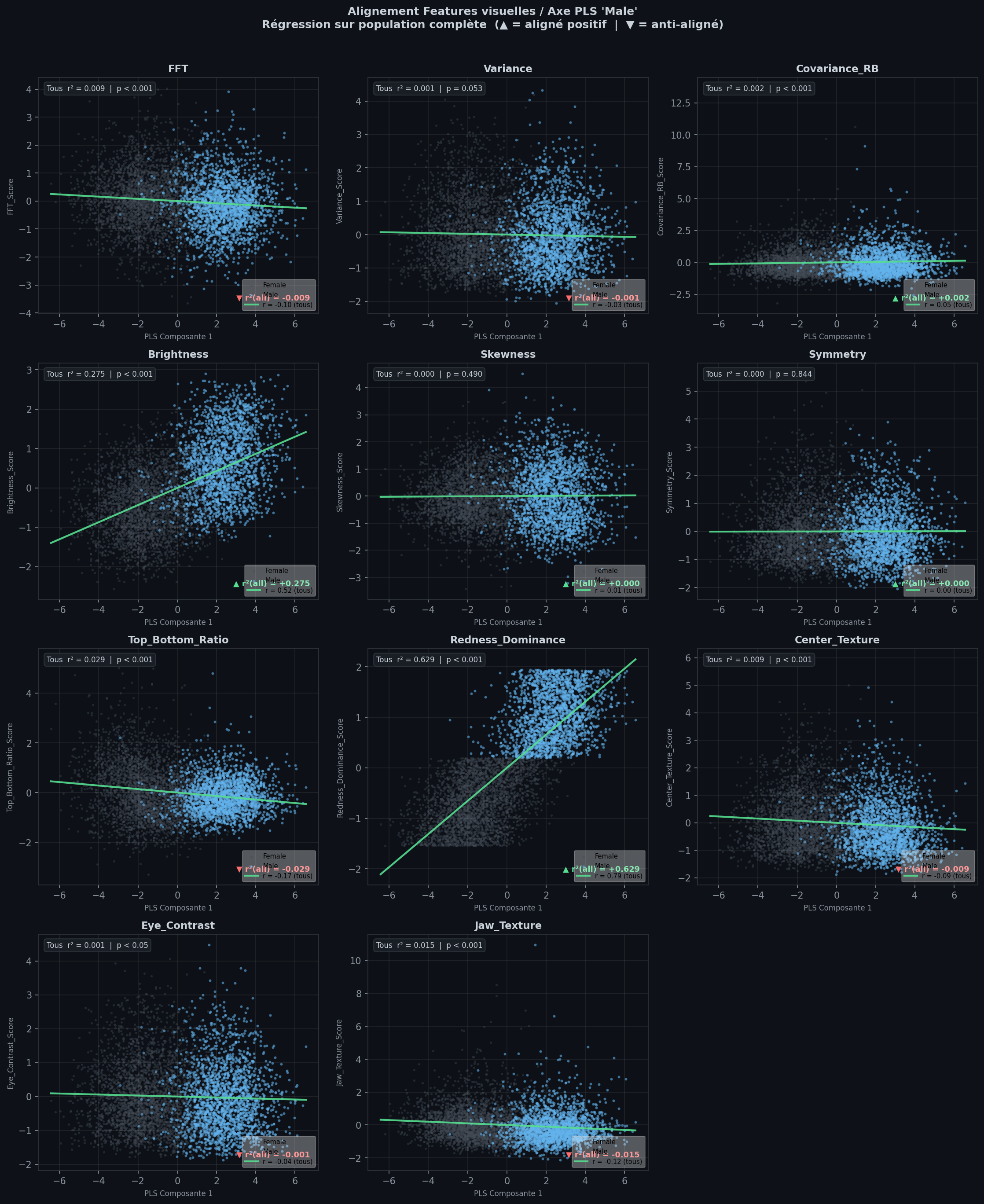
Reading the alignment panels
Each panel plots PLS component 1 (horizontal, latent direction linked to your classes) against one standardized feature score on the vertical axis (each column from compute_feature_score_table is scaled to mean 0 and standard deviation 1 over your sample, so brightness, texture, etc. are comparable on the same plot grid).
| Element | Meaning |
|---|---|
| Grey / blue points | Class B / class A |
| Green line | Linear trend across all points; legend shows Pearson r |
| Top-left | Strength of association (|r²|) and regression p-value |
| ▲ / ▼ signed r² | Feature increases or decreases when PLS1 moves toward class A (target_label) |
Two extremes cases
1. Horizontal green line — weak link to classification
The regression line is flat and the cloud does not climb or fall along PLS1. The feature co-varies little with this latent axis: the model is probably not using this cue to distinguish the two classes (e.g. skewness, symmetry in the example above).
2. Diagonal green line — captured bias
Points spread along a clear slope: low PLS1 ↔︎ low feature value on one side, high PLS1 ↔︎ high value on the other. Class A and class B often separate left–right and bottom–top. That is a strong sign that the model may rely on this pixel-level cue to classify (e.g. redness_dominance, brightness in the example figure, with class A = Male and class B = Female).
Use the panels to confirm features that stand out in the importance ranking, not to rank them (that is the bar chart’s job).
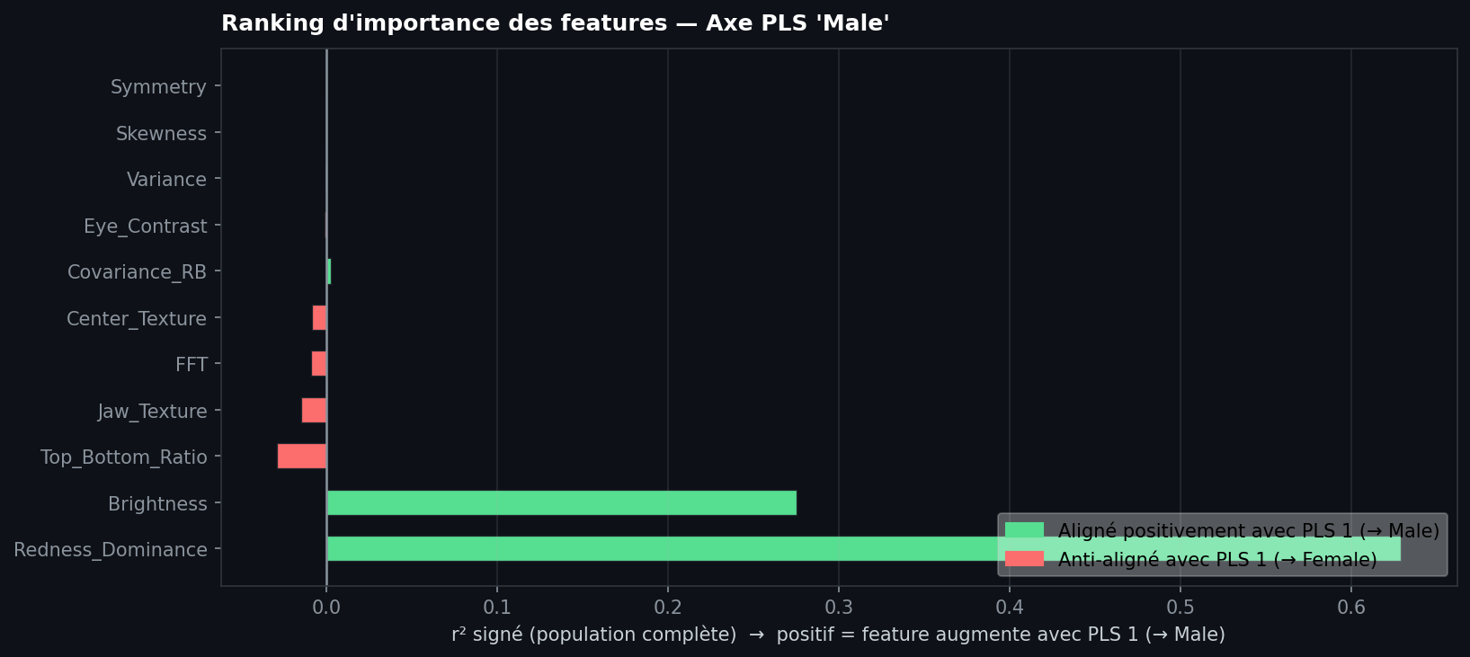
Reading the importance ranking
One horizontal bar per feature, sorted by |signed r²| with PLS component 1 (strongest at the top).
| Element | Meaning |
|---|---|
| Green bar (right) | Feature increases with PLS1 toward class A (target_label) |
| Red bar (left) | Feature decreases when PLS1 moves toward class A (anti-aligned → class B) |
| Bar length | Strength of linear association (not a p-value) |
| Near-zero bar | Little linear coupling to the latent axis on the full sample |
How to read the chart
- Top of the list: Features most aligned with the latent decision axis — start here when asking what the model might use in image space.
- Long green bars: Cues that rise with PLS1 toward class A; open the matching alignment panel — you should see a diagonal green line and separated classes.
- Short or near-zero bars: Weak linear link to the latent axis; the corresponding alignment panel usually shows a horizontal green line and a mixed cloud.
- Compare with alignment panels: The ranking is a compact summary; the grid validates whether a large bar reflects a real visual bias or an outlier-driven slope.
Reading the example figure
On this human gender classification (class A = Male, class B = Female), the chart suggests the latent classification axis is mostly carried by color and luminance, not by shape regularity:
- Strong cues: redness_dominance and brightness have the longest green bars (high signed r²). The model’s PLS1 direction co-varies strongly with “more red” and “brighter” toward class A — plausible pixel-level biases for this task.
- Weak cues: symmetry_error, skewness, variance, and eye_region_contrast have bars close to zero. Along PLS1, facial symmetry (and these other scores) show little linear association with the classification axis in this sample — not evidence that the model relied on them here.
This is a hypothesis from alignment statistics, not a proof of what the network computes internally. Always cross-check the alignment panels for the top features.
Use this figure for reporting and comparing runs; use the alignment panels for qualitative checks on the top features.
run_pls_feature_figures
def run_pls_feature_figures(
    z:np.ndarray, target_score:np.ndarray, feature_table, feature_columns:Sequence[str] | None=None,
    target_label:str='target', mask_positive:np.ndarray | None=None, positive_label:str='positive',
    negative_label:str='negative', save_dir:str | Path | None=None, show:bool=True
)->dict[str, Any]:
Build alignment panels and importance ranking; display and optionally save PNGs.