# Classification Interpretation


<!-- WARNING: THIS FILE WAS AUTOGENERATED! DO NOT EDIT! -->

After **`train_xaaenet`**, compare the model’s latent codes to
interpretable pixel scores: latent matrix `z` (one row per image) and a
feature table from `compute_feature_score_table`, on the **same images
in the same order**. For **binary** classification, encode one level as
class **A** (`target_score = 1.0`) and the other as class **B** (`0.0`).

Call **`run_pls_feature_figures`** to build, display, and optionally
save two figures:

1.  **Alignment panels** — one scatter plot per feature (latent axis vs
    feature value);
2.  **Importance ranking** — bars ranked by how strongly each feature
    follows that axis.

A full end-to-end example lives in the tutorial notebook.

## `run_pls_feature_figures`

``` python
from tell_me_why.feature_scores import compute_feature_score_table
from tell_me_why.visualization import run_pls_feature_figures

# z: (n_images, latent_dim) from your trained xAAEnet on the split you analyse
# target_score: 1.0 = class A, 0.0 = class B, same row order as z
df_features = compute_feature_score_table([str(p) for p in image_paths])

out = run_pls_feature_figures(
    z,
    target_score,
    df_features,
    target_label="A",
    mask_positive=target_score.astype(bool),  # True for class A
    positive_label="A",
    negative_label="B",
    save_dir="results/pls",
    show=True,
)

fig_panels = out["alignment_fig"]
fig_ranking = out["importance_fig"]
ranked_features = out["importance_rank"]
```

### Arguments

<table>
<colgroup>
<col style="width: 62%" />
<col style="width: 37%" />
</colgroup>
<thead>
<tr>
<th>Argument</th>
<th>Role</th>
</tr>
</thead>
<tbody>
<tr>
<td><code>z</code></td>
<td>Latent codes from your trained model: one row per image, shape
<code>(number of images, latent dimension)</code> — e.g. 500 images ×
128-D latent space → <code>(500, 128)</code></td>
</tr>
<tr>
<td><code>target_score</code></td>
<td>Binary targets: <code>1.0</code> = class A, <code>0.0</code> = class
B</td>
</tr>
<tr>
<td><code>feature_table</code></td>
<td>DataFrame from <code>compute_feature_score_table</code></td>
</tr>
<tr>
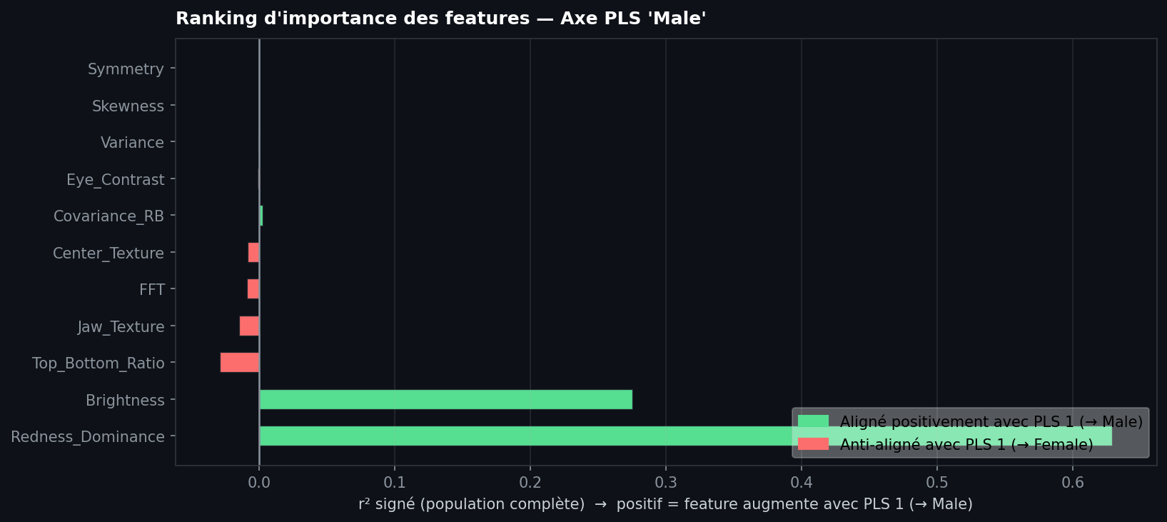
<td><code>target_label</code></td>
<td>Name of class A on the importance chart</td>
</tr>
<tr>
<td><code>mask_positive</code></td>
<td>Boolean mask where <code>target_score == 1.0</code> (class A)</td>
</tr>
<tr>
<td><code>positive_label</code>, <code>negative_label</code></td>
<td>Legend labels for class A and class B on alignment panels</td>
</tr>
<tr>
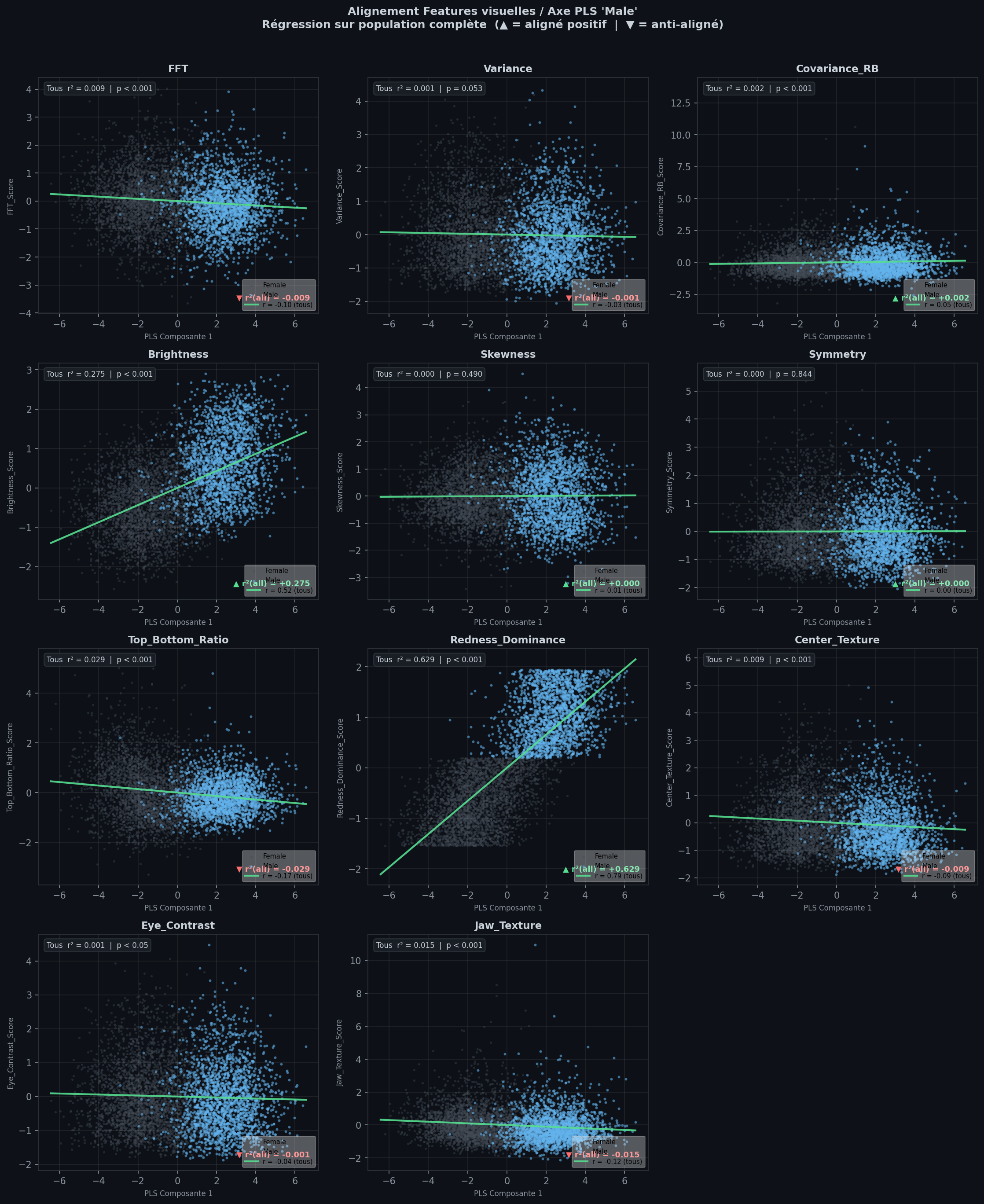
<td><code>feature_columns</code></td>
<td>Columns to plot (default: all eleven feature scores)</td>
</tr>
<tr>
<td><code>save_dir</code></td>
<td>Saves <code>feature_alignment_panels.png</code> and
<code>feature_importance_ranking.png</code></td>
</tr>
<tr>
<td><code>show</code></td>
<td>Call <code>plt.show()</code> for each figure (<code>False</code>
keeps figures only in <code>out</code>)</td>
</tr>
</tbody>
</table>

## Reading the alignment panels

Each panel plots **PLS component 1** (horizontal, latent direction
linked to your classes) against one **standardized feature score** on
the vertical axis (each column from `compute_feature_score_table` is
scaled to mean 0 and standard deviation 1 over your sample, so
brightness, texture, etc. are comparable on the same plot grid).

<figure>
<img src="images/feature_alignment_panels_example.png"
alt="Feature alignment panels — binary example (class A vs class B)" />
<figcaption aria-hidden="true">Feature alignment panels — binary example
(class A vs class B)</figcaption>
</figure>

<table>
<colgroup>
<col style="width: 52%" />
<col style="width: 47%" />
</colgroup>
<thead>
<tr>
<th>Element</th>
<th>Meaning</th>
</tr>
</thead>
<tbody>
<tr>
<td>Grey / blue points</td>
<td>Class B / class A</td>
</tr>
<tr>
<td>Green line</td>
<td>Linear trend across all points; legend shows Pearson
<code>r</code></td>
</tr>
<tr>
<td>Top-left</td>
<td>Strength of association (<code>|r²|</code>) and regression
p-value</td>
</tr>
<tr>
<td>▲ / ▼ signed r²</td>
<td>Feature increases or decreases when PLS1 moves toward class A
(<code>target_label</code>)</td>
</tr>
</tbody>
</table>

### Two extremes cases

**1. Horizontal green line — weak link to classification**

The regression line is flat and the cloud does not climb or fall along
PLS1. The feature co-varies little with this latent axis: the model is
probably **not** using this cue to distinguish the two classes
(e.g. *skewness*, *symmetry* in the example above).

**2. Diagonal green line — captured bias**

Points spread along a clear slope: low PLS1 ↔ low feature value on one
side, high PLS1 ↔ high value on the other. Class A and class B often
separate left–right **and** bottom–top. That is a strong sign that the
model may **rely on this pixel-level cue** to classify
(e.g. *redness_dominance*, *brightness* in the example figure, with
class A = Male and class B = Female).

Use the panels to **confirm** features that stand out in the importance
ranking, not to rank them (that is the bar chart’s job).

## Reading the importance ranking

One horizontal bar per feature, sorted by **|signed r²|** with PLS
component 1 (strongest at the top).

<figure>
<img src="images/feature_importance_ranking_example.png"
alt="Feature importance ranking — binary example (class A vs class B)" />
<figcaption aria-hidden="true">Feature importance ranking — binary
example (class A vs class B)</figcaption>
</figure>

<table>
<colgroup>
<col style="width: 52%" />
<col style="width: 47%" />
</colgroup>
<thead>
<tr>
<th>Element</th>
<th>Meaning</th>
</tr>
</thead>
<tbody>
<tr>
<td>Green bar (right)</td>
<td>Feature increases with PLS1 toward class A
(<code>target_label</code>)</td>
</tr>
<tr>
<td>Red bar (left)</td>
<td>Feature decreases when PLS1 moves toward class A (anti-aligned →
class B)</td>
</tr>
<tr>
<td>Bar length</td>
<td>Strength of linear association (not a p-value)</td>
</tr>
<tr>
<td>Near-zero bar</td>
<td>Little linear coupling to the latent axis on the full sample</td>
</tr>
</tbody>
</table>

### How to read the chart

- **Top of the list:** Features most aligned with the latent decision
  axis — start here when asking what the model might use in image space.
- **Long green bars:** Cues that rise with PLS1 toward class A; open the
  matching alignment panel — you should see a **diagonal** green line
  and separated classes.
- **Short or near-zero bars:** Weak linear link to the latent axis; the
  corresponding alignment panel usually shows a **horizontal** green
  line and a mixed cloud.
- **Compare with alignment panels:** The ranking is a compact summary;
  the grid validates whether a large bar reflects a real visual bias or
  an outlier-driven slope.

### Reading the example figure

On this human gender classification (class A = Male, class B = Female),
the chart suggests the latent classification axis is **mostly carried by
color and luminance**, not by shape regularity:

- **Strong cues:** *redness_dominance* and *brightness* have the longest
  green bars (high signed r²). The model’s PLS1 direction co-varies
  strongly with “more red” and “brighter” toward class A — plausible
  pixel-level biases for this task.
- **Weak cues:** *symmetry_error*, *skewness*, *variance*, and
  *eye_region_contrast* have bars close to zero. Along PLS1, facial
  symmetry (and these other scores) show **little linear association**
  with the classification axis in this sample — not evidence that the
  model relied on them here.

This is a **hypothesis from alignment statistics**, not a proof of what
the network computes internally. Always cross-check the alignment panels
for the top features.

Use this figure for reporting and comparing runs; use the alignment
panels for qualitative checks on the top features.

------------------------------------------------------------------------

### run_pls_feature_figures

``` python

def run_pls_feature_figures(
    z:np.ndarray, target_score:np.ndarray, feature_table, feature_columns:Sequence[str] | None=None,
    target_label:str='target', mask_positive:np.ndarray | None=None, positive_label:str='positive',
    negative_label:str='negative', save_dir:str | Path | None=None, show:bool=True
)->dict[str, Any]:

```

*Build alignment panels and importance ranking; display and optionally
save PNGs.*