from pathlib import Path

from fastai.vision.all import URLs, get_image_files, untar_data
from PIL import Image
import matplotlib.pyplot as pltFeature Scores
Utility functions for mapping fastai learner outputs and computing interpretable scores on images.
Walkthrough: PETS in a few cells
This opening section runs end-to-end on a small slice of the fastai Oxford-IIIT Pet dataset so you can see concrete numeric outputs before reading the API reference below.
Only the first 8 images returned by get_image_files are used so the documentation remains quick to generate. The goal is not to analyze the full dataset here, but to show real compute_feature_score_table output on disk files.
# Import a dataset (example: fastai PETS).
pets_path = untar_data(URLs.PETS) / "images"
pet_images = list(get_image_files(pets_path))[:8]len(pet_images), [path.name for path in pet_images](8,
['shiba_inu_14.jpg',
'Bombay_58.jpg',
'Siamese_173.jpg',
'miniature_pinscher_4.jpg',
'beagle_31.jpg',
'chihuahua_75.jpg',
'Bengal_58.jpg',
'Russian_Blue_130.jpg'])# Uses the installed package so this walkthrough can appear before the `#| export` cells.
import tell_me_why.feature_scores as _fs
pets_scores = _fs.compute_feature_score_table(
pet_images,
score_names=[
"brightness",
"variance",
"redness_dominance",
"symmetry_error",
"fft_high_frequency_ratio",
],
on_error="raise",
)
pets_scores_display = pets_scores.copy()
pets_scores_display["image_name"] = pets_scores_display["Source_File_Path"].map(lambda path: Path(path).name)
pets_scores_display = pets_scores_display.drop(columns="Source_File_Path")
pets_scores_display = pets_scores_display[["image_name", *[col for col in pets_scores_display.columns if col != "image_name"]]]
pets_scores_display.round(4)
Computing brightness:   0%|          | 0/8 [00:00<?, ?it/s]
Computing brightness: 100%|##########| 8/8 [00:00<00:00, 627.75it/s]

Computing variance / contrast:   0%|          | 0/8 [00:00<?, ?it/s]
Computing variance / contrast: 100%|##########| 8/8 [00:00<00:00, 646.05it/s]

Computing red dominance:   0%|          | 0/8 [00:00<?, ?it/s]
Computing red dominance: 100%|##########| 8/8 [00:00<00:00, 432.94it/s]

Computing symmetry:   0%|          | 0/8 [00:00<?, ?it/s]
Computing symmetry: 100%|##########| 8/8 [00:00<00:00, 615.72it/s]

Computing FFT scores:   0%|          | 0/8 [00:00<?, ?it/s]
Computing FFT scores: 100%|##########| 8/8 [00:00<00:00, 406.85it/s]| image_name | brightness | variance | redness_dominance | symmetry_error | fft_high_frequency_ratio | |
|---|---|---|---|---|---|---|
| 0 | shiba_inu_14.jpg | 0.7555 | 0.0176 | 0.5491 | 0.0889 | 0.5315 |
| 1 | Bombay_58.jpg | 0.1711 | 0.0477 | 0.7016 | 0.1534 | 0.4465 |
| 2 | Siamese_173.jpg | 0.4284 | 0.0479 | 0.5613 | 0.2105 | 0.5394 |
| 3 | miniature_pinscher_4.jpg | 0.5688 | 0.0625 | 0.5165 | 0.2563 | 0.4899 |
| 4 | beagle_31.jpg | 0.4799 | 0.0355 | 0.4072 | 0.2172 | 0.6502 |
| 5 | chihuahua_75.jpg | 0.4795 | 0.0594 | 0.7384 | 0.2793 | 0.4448 |
| 6 | Bengal_58.jpg | 0.6254 | 0.0477 | 0.5762 | 0.2379 | 0.4307 |
| 7 | Russian_Blue_130.jpg | 0.5452 | 0.0665 | 0.5519 | 0.1784 | 0.4253 |
fig, axes = plt.subplots(2, 4, figsize=(10, 5))

for ax, image_path in zip(axes.flat, pet_images):
    ax.imshow(Image.open(image_path))
    ax.set_title(image_path.stem[:18], fontsize=8)
    ax.axis("off")

plt.tight_layout()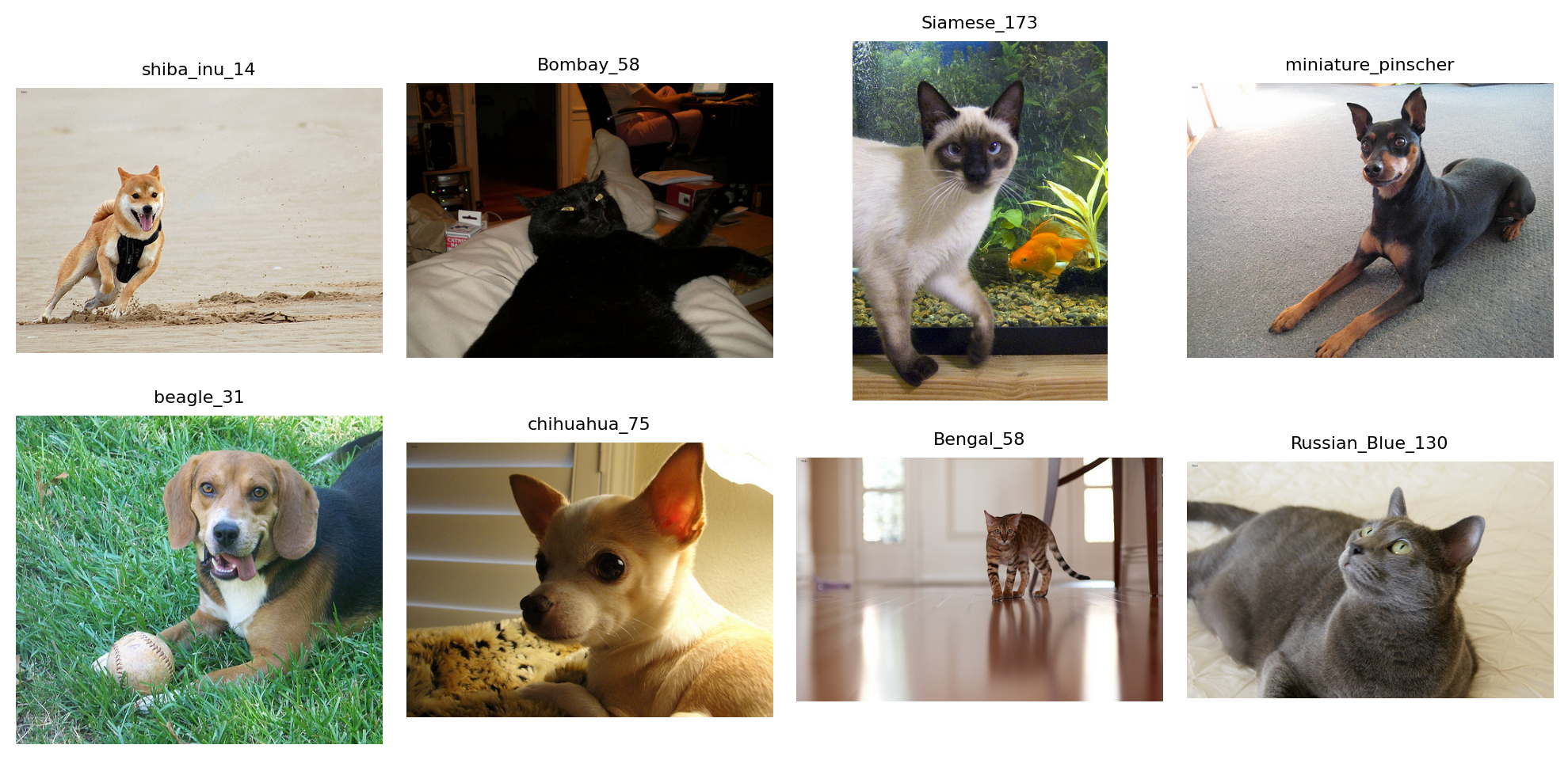
The values obtained here are not interpreted as model explanations. They are used to verify that each score family produces a numeric measurement on real images:
brightnessandvariancedescribe global intensity;redness_dominancecomes from the color family;symmetry_errorcomes from the spatial family;fft_high_frequency_ratiocomes from the frequency family.
The sections below document every helper behind this table, including map_learner_predictions for aligning paths with fastai learner outputs.
Mapping Learner Outputs
Before comparing feature scores with model predictions, the alignment between learner outputs and the original files must be preserved. The following function keeps the order produced by get_preds(..., reorder=False) and reconstructs a provenance table.
map_learner_predictions
def map_learner_predictions(
    learn:Any, # Learner whose dataloaders expose the original dataset items.
    ds_idxs:Sequence[int]=(0, 1), # Dataset indices to map. In fastai, 0 is usually train and 1 is valid.
    include_predictions:bool=False, # When True, append target and prediction columns to the provenance table.
): # Concatenated inputs and a DataFrame aligned row-by-row with these inputs.
Map fastai learner predictions back to their source files.
Global Intensity Scores
These scores summarize the grayscale distribution across the whole image. They are useful for detecting brightness, contrast, or statistical asymmetry effects that can influence a binary classifier without directly corresponding to semantic structure.
compute_skewness_scores
def compute_skewness_scores(
    image_paths:Iterable[ImagePath], on_error:ErrorPolicy='previous'
)->list[float]:
Compute grayscale skewness for each image.
compute_variance_scores
def compute_variance_scores(
    image_paths:Iterable[ImagePath], on_error:ErrorPolicy='previous'
)->list[float]:
Compute grayscale variance as a global contrast score.
compute_brightness_scores
def compute_brightness_scores(
    image_paths:Iterable[ImagePath], on_error:ErrorPolicy='previous'
)->list[float]:
Compute mean grayscale intensity for each image.
Color Scores
These scores use the RGB channels. They should be interpreted carefully: they can capture dataset, lighting, makeup, or preprocessing effects as much as cues that are truly related to the class.
compute_redness_dominance_scores
def compute_redness_dominance_scores(
    image_paths:Iterable[ImagePath], on_error:ErrorPolicy='previous'
)->list[float]:
Compute red-channel dominance relative to green and blue channels.
compute_color_covariance_scores
def compute_color_covariance_scores(
    image_paths:Iterable[ImagePath], on_error:ErrorPolicy='previous'
)->list[float]:
Compute covariance between red and blue channels.
Spatial and Regional Scores
These scores preserve positional information: left-right symmetry, top/bottom ratio, central texture, eye-band contrast, and edge activity in the jaw region. They are closer to visual hypotheses about faces, so they are less generic than global scores.
compute_jaw_texture_scores
def compute_jaw_texture_scores(
    image_paths:Iterable[ImagePath], on_error:ErrorPolicy='previous'
)->list[float]:
Compute lower-face edge activity from adjacent-pixel intensity differences.
compute_eye_region_contrast_scores
def compute_eye_region_contrast_scores(
    image_paths:Iterable[ImagePath], on_error:ErrorPolicy='previous'
)->list[float]:
Compute grayscale variance in a horizontal band roughly matching the eye region.
compute_center_texture_scores
def compute_center_texture_scores(
    image_paths:Iterable[ImagePath], on_error:ErrorPolicy='previous'
)->list[float]:
Compute grayscale variance in the central crop of each image.
compute_top_bottom_ratio_scores
def compute_top_bottom_ratio_scores(
    image_paths:Iterable[ImagePath], on_error:ErrorPolicy='previous'
)->list[float]:
Compute mean brightness ratio between upper and lower halves.
compute_symmetry_scores
def compute_symmetry_scores(
    image_paths:Iterable[ImagePath], on_error:ErrorPolicy='previous'
)->list[float]:
Compute horizontal symmetry error. Lower values mean stronger symmetry.
Frequency Scores and Thresholds
Frequency scores move into the Fourier domain to measure the proportion of energy carried by high frequencies. The Otsu helper remains separate: it does not directly produce a dataset score, but can be used to build scores based on segmentation or foreground/background separation.
find_otsu_threshold
def find_otsu_threshold(
    im_gray:Tensor
)->int:
Find Otsu’s threshold for a grayscale image tensor.
Accepts images scaled either in [0, 1] or [0, 255].
compute_fft_scores
def compute_fft_scores(
    image_paths:Iterable[ImagePath], radius:int=30, image_size:tuple[int, int]=(200, 200),
    on_error:ErrorPolicy='previous'
)->list[float]:
Compute the high-frequency energy ratio for each image.
The central disk of radius radius is treated as low frequency. The score is the remaining high-frequency energy divided by total FFT magnitude energy.
Exported Catalog
The registry below provides a common API for listing available scores or computing a complete table. Keys remain in English for the Python API, while the notebook sections document the intent of each category.
compute_feature_score_table
def compute_feature_score_table(
    image_paths:Iterable[ImagePath], # Images to score.
    score_names:Sequence[str] | None=None, # Names from `available_feature_scores()`. When omitted, all scores are computed.
    on_error:ErrorPolicy='previous', # Error handling policy for unreadable images.
):
Compute selected feature scores and return them in a pandas DataFrame.
available_feature_scores
def available_feature_scores(

)->dict[str, list[str]]:
Return available feature-score names grouped by category.